Marine Sediment Characterized by Ocean-Bottom Fiber-Optic Seismology
Marine Sediment Characterized by Ocean-Bottom Fiber-Optic Seismology
Spica, Z. J., Nishida, K., Akuhara, T., Pétrélis, F., Shinohara, M., & Yamada, T. (2020). Marine sediment characterized by ocean‐bottom fiber‐optic seismology. Geophysical Research Letters, 47, e2020GL088360. https://doi.org/10.1029/2020GL088360
Abstract The Sanriku ocean‐bottom seismometer system uses an optical fiber cable to guarantee real‐time observations at the seafloor. A dark fiber connected to a Distributed Acoustic Sensing (DAS) interrogator converted the cable in an array of 19,000 seismic sensors. We use these measurements to constrain the velocity structure under a section of the cable. Our analysis relies on 24 hr of ambient seismic field recordings. We obtain a high‐resolution 2‐D shear‐wave velocity profile by inverting multimode dispersion curves extracted from frequency‐wave number analysis. We also produce a reflection image from autocorrelations of ambient seismic field, highlighting strong impedance contrasts at the interface between the sedimentary layers and the basement. In addition, earthquake wavefield analysis and modeling help to further constrain the sediment properties under the cable. Our results show for the first time that ocean‐bottom DAS can produce detailed images of the subsurface, opening new opportunities for cost‐effective ocean‐bottom imaging in the future.
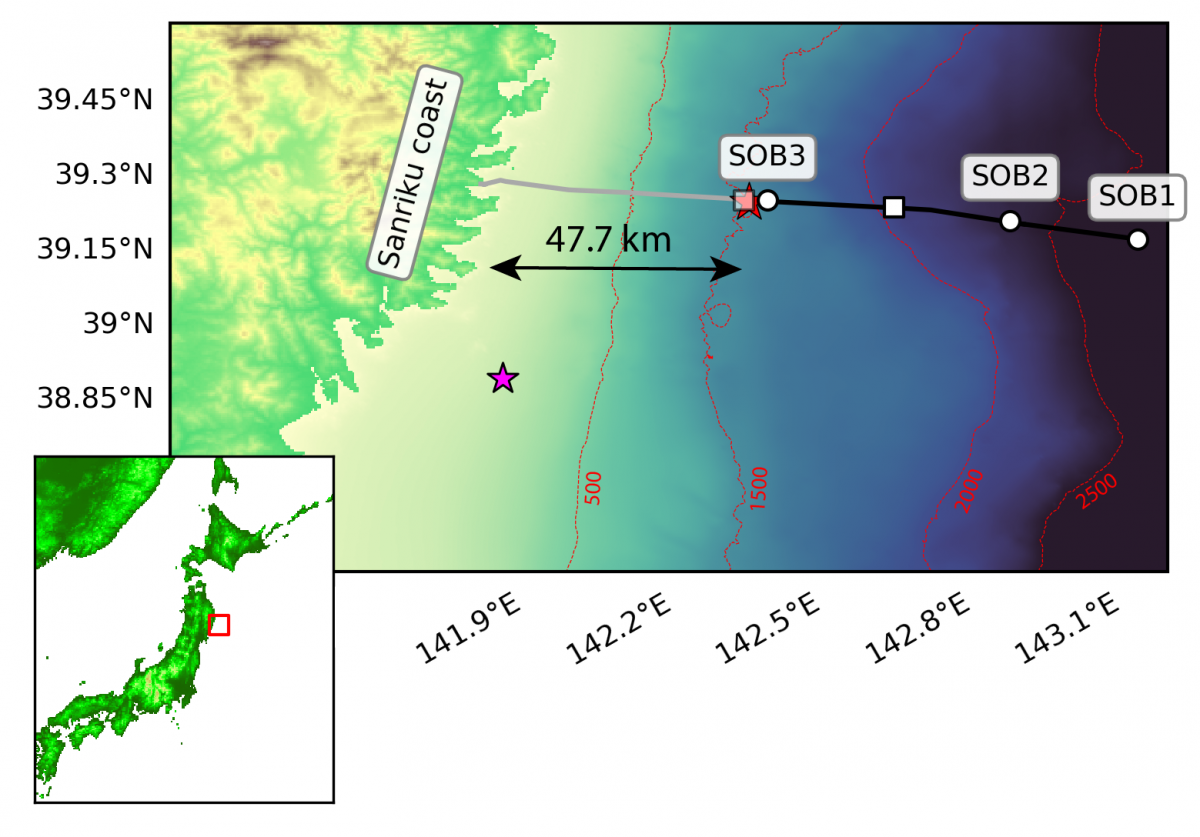
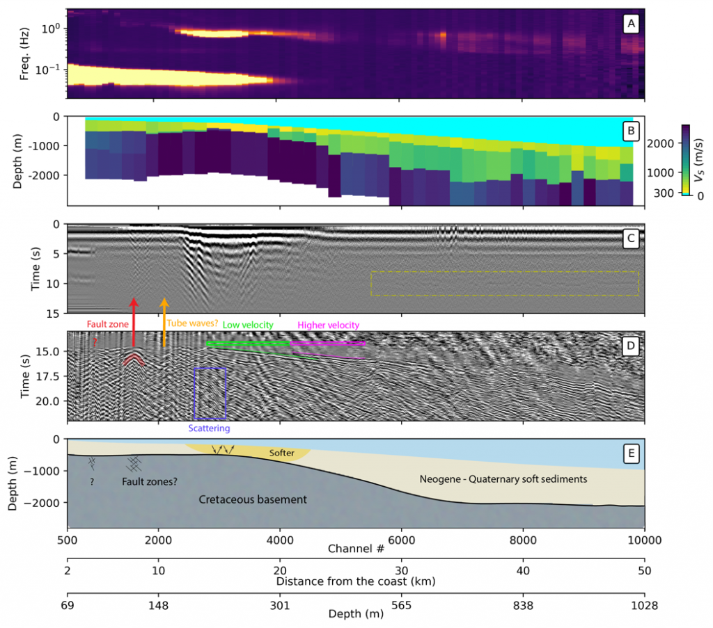
Map showing the location of the telecommunication fiber‐optic cable off the shore of Sanriku. The gray section of the cable, which is used in our analyses, is buried under 60–70 cm of sediment, while the black section lies directly on the seafloor by gravity. The white dots depict the accelerometers, and the white squares are the pressure gauges. The pink star depicts the location of an earthquake (2019‐02‐14T21:10:50; Mw = 3.0) recorded by DAS and shown in Figure 3c. The red star depicts the location of another earthquake recorded only by the OBS systems (2018‐01‐30T17:20:56.31; Mw = 3.1; depth = 30.9 km) and showed in Figure 4. (a) Power spectral densities along the cable every 500 channel, as shown in Figure 2a (oceanward). (b) Two‐dimensional shear‐wave velocity profile obtained from the inversion of the dispersion curves at each subset of 1,000 channels, as shown in Figure S3. (c) Reflection image from autocorrelations of ASF. All autocorrelation functions are band‐pass filtered between 0.8 and 4.5 Hz. The yellow box highlights potential velocity contrast corresponding to a four‐way travel time reflected S waves. A zoom in the yellow box is shown in Figure S4d. (d) S wave arrivals with automatic gain control for an earthquake recorded by the array as shown in Figure 1. In the green area, the S wave arrives after the S wave in the purple area, which suggests a lower velocity zone. The inverted V shapes that may characterize fault zones are highlighted with a red arrow and a red question mark. These fault‐zone regions are sometimes associated with amplification effects observed in the autocorrelation functions. Other amplification or scattering effects (orange arrow and blue box) may also be explained by localized tube waves or basin‐edge scattering. (e) Geological interpretation that combines the observations of all panels.